The DTFT and the Sampling Theorem

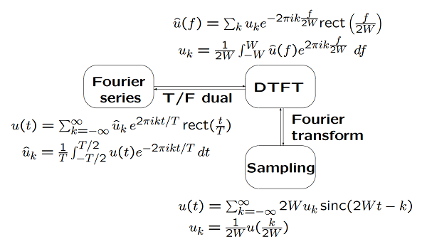
Posted May 04, 2017 | View revision history

The discrete-time Fourier transform (DTFT) is the time/frequency dual of the Fourier series. In the sense of $L^2$ convergence, Fourier series uses the sequence of coefficients to represent the function, DTFT uses the frequency function to represent the sequence. DTFT is similar to modulation from discrete to waveform.

The Discrete-time Fourier Transform

Familiar DTFT expression

$$x[n] = {1 \over 2\pi} \int_{2\pi} X(\Omega) e^{j\Omega n} d\Omega = {1 \over 2\pi} \int_{2\pi} X(e^{j\omega n}) e^{j\omega n} d\omega \tag{synthesis}$$ $$X(\Omega) = X(e^{j\omega n}) = \sum\limits_{-\infty}^{\infty} x[n]e^{-j\omega n} = \sum\limits_{-\infty}^{\infty} x[n]e^{-j\Omega n} \tag{analysis}$$

DTFT

Assume $\{\hat u(f) : [-W, W] \to \Bbb C \}$ is $L^2$ (and thus also $L^1$). The DTFT of $\hat u(f)$ over $[−W,W]$ is then defined by

$$\hat u(f) = l.i.m. \sum\limits_k u_k e^{-2\pi ikf/(2W)} rect(f/2W)$$

where the DTFT coefficients $\{u_k; k \in \Bbb Z\}$ are given by

$$u_k = {1 \over 2W} \int_{-W}^{W} \hat u(f)e^{2\pi i kf/(2W)} df \tag {1}$$

We also write this as

$$\hat u(f) = l.i.m. \sum\limits_k u_k \hat {\phi}_k(f) \tag{2}$$

where,

$$\hat {\phi}_k(f) = e^{-2 \pi ikf/(2W)} rect(f/2W)$$

DTFT theorem

Let $\{\hat u(f) : [-W, W] \to \Bbb C \}$ be an $L^2$. Then for each $k \in \Bbb Z$, the Lebesgue integral $(1)$ exists and satisfies $|u_k| \le {1 \over 2W} \int |\hat u(f)|df \lt \infty$. Furthermore,

$$\lim_{\ell \to \infty}\int_{-W}^{W}|\hat u(f) - \sum\limits_{k=-\ell}^{\ell} u_k e^{-2 \pi ikf/(2W)}|^2 df = 0 \tag{3}$$ $$\int_{-W}^{W} |\hat u(f)| df = 2W \sum\limits_{-\infty}^{\infty}|u_k|^2 \tag{4}$$

Finally, if $\{u_k; k \in \Bbb Z\}$ is a sequence of complex numbers satisfying $\sum_k |u_k|^2 < \infty$, then an $L^2$ function $\{\hat u(f) : [-W, W] \to \Bbb C \}$ exists satisfying $(3)$ and $(4)$.

The sampling theorem

$\hat u(f)$ for an L2 baseband waveform is both $L^1$ and $L^2$. Thus, at every $t$

$$u(t) = \int_{-W}^W \hat u(f) e^{2\pi ift}df$$

and $u(t)$ is continuous. Since the transform pair

$$rect({f \over 2W}) \leftrightarrow 2Wsinc(2Wt) \tag{scaling relation}$$

the inverse transform of $\hat \phi_k(f)$ is

$$\phi_k(t) = 2Wsinc(2Wt-k) \leftrightarrow \hat \phi_k(f) = e^{-2\pi ikf/(2W)}rect(f/2W) \tag{time-shift relation} $$

Then

$$u(t) = \sum\limits_k u_k \phi_k(t) = \sum\limits_k 2W u_k sinc(2Wt-k) = \sum\limits_{k=-\infty}^{\infty} u(k/2W) sinc(2Wt-k) \tag{5}$$

Sampling theorem

Let $\{\hat u(f) : [-W, W] \to \Bbb C \}$ be $L^2$ (and thus also $L^1$). For $u(t)$ in (5), let $T = 1/(2W)$. Then $u(t)$ is continuous, $L^2$, and bounded by $u(t) \le \int_{-W}^W |\hat u(f)| df$. Also, for all $t \in \Bbb R$,

$$u(t) = \sum\limits_{-\infty}^{\infty}u(kT) sinc({t-kT \over T})$$

This says that a baseband-limited function is specified by its samples intervals $T = 1/(2W)$.
The sinc function is nonzero over all noninteger times. Recreating the waveform at the receiver from a set of samples thus requires infinite delay(band-limited functions are not time-limited).
Practically sinc functions can be truncated, but the sinc waveform decays to zero as $1/t$, which is impractically slow.

Baseband-limited

An $L^2$ function is baseband-limited to $W$ if it is the pointwise inverse transform of an $L^2$ function $\hat u(f)$ that is 0 for $|f| > W$. Equivalently, it is baseband-limited to $W$ if it is continuous and its Fourier transform is 0 for $|f| > 0$.
There are other bandlimited functions, limited to $[−W, W]$, which are not continuous. The sampliing theorem does not hold for these functions.
DTFT

The sampling theorem for $[\Delta −W, \Delta+W]$

Consider an $L^2$ frequency function $\{\hat v(f) : [\Delta −W, \Delta +W] \to \Bbb C\}$. The shifted DTFT for $\hat v(f)$ is then

$$\hat v(f) = l.i.m. \sum\limits_k v_k e^{-2\pi ikf/(2W)} rect({f-\Delta \over 2W}) = l.i.m. \sum\limits_k v_k \hat \theta_k(f)$$

where

$$v_k = {1 \over 2W} \int_{\Delta -W}^{\Delta +W} \hat v(f)e^{2\pi i kf/(2W)} df$$
The inverse Fourier transform of $\hat \theta_k(f)$ can be calculated by shifting and scaling to be

$$\theta_k(t) = 2Wsinc(2Wt-k)e^{2\pi i\Delta(t-{k \over 2W})} \leftrightarrow \hat \theta_k(f) = e^{-2\pi ikf/(2W)}rect({f-\Delta \over 2W})$$

This generalizes the sampling equation to the frequency band $[\Delta −W, \Delta +W]$, let $T=1/2W$,

$$v(t) = \sum\limits_k v_k \theta_k(t) = \sum\limits_k v({k \over 2W}) sinc(2Wt-k)e^{2\pi i\Delta(t-{k \over 2W})} = \sum\limits_k v({kT}) sinc({t \over T}-k)e^{2\pi i\Delta(t-kT)}$$

Reference:

Robert Gallager. (2006). 6.450 Digital Communication. MIT OpenCourseWare (http://ocw.mit.edu/)
Robert G.Gallager. (2009). Principles of Digital Communication (New York: Cambridge University Press).
Alan V.Oppenheim. Alan S.Willsky. (1998). Signals and systems 2nd ed. (China: Prentice-Hall International,Inc).
Shlomo Engelberg. (2008). Digital Signal Processing An Experimental Approach. (Springer-Verlag London Limited).

A good person! More about the author →